Get Started

Diffusion model has been widely used in generative AI, especially in the vision domain. In our paper, we proposed RegDiffusion, a diffusion based model for GRN inference. Compared with previous model, RegDiffusion completes inference within a fraction of time and yield better benchmarking results.

In this tutorial, we provide an example of running GRN inference using RegDiffusion and generating biological insights from the inferred network.

Requirements

We will need the python package regdiffusion for GRN inference. For accelerated inference speed, you may want to run regdiffusion on GPU devices with the latest CUDA installation.

>>> import regdiffusion as rd
>>> import numpy as numpy

Data Loading

The input of regdiffusion is simply a single-cell gene expression matrix, where the columns are genes and rows are cells. We expect you to log transform your data. RegDiffusion is capable to infer GRNs among 10,000+ genes (depending on GPU hardware) within minutes so there is no need to apply heavy gene filtering. The only genes you may want to remove are genes that are not expressed at all (total raw count on all cells == 0).

The regdiffusion package comes with a set of preprocessed data, including the BEELINE benchmarks, Hammond microglia in male adult mice, and another labelled microglia subset from a mice cerebellum atlas project.

Here we use the mESC data from the BEELINE benchmark. The mESC data comes from Mouse embryonic stem cells. It has 421 cells and 1,620 genes.

If you want to see the inference on a larger network with 14,000+ genes and 8,000+ cells, check out the other example.

>>> bl_dt, bl_gt = rd.data.load_beeline(
>>>     benchmark_data='mESC', benchmark_setting='1000_STRING'
>>> )

Here, load_beeline gives you a tuple, where the first element is an anndata of the single cell experession data and the second element is an array of all the ground truth links (based on the STRING network in this case).

>>> bl_dt
AnnData object with n_obs × n_vars = 421 × 1620
    obs: 'cell_type', 'cell_type_index'

>>> bl_gt
array([['KLF6', 'JUN'],
       ['JUN', 'KLF6'],
       ['KLF6', 'ATF3'],
       ...,
       ['SIN3A', 'TET1'],
       ['MEF2C', 'TCF12'],
       ['TCF12', 'MEF2C']], dtype=object)

GRN Inference

You are recommended to use the provided trainer to train a RegDiffusion Model. You need to provide the expression data in a numpy array to the trainer.

During the training process, the training loss and the average amount of change on the adjacency matrix are provided on the progress bar. The model converges when the step change n the adjacency matrix is near-zero. By default, the train method will train the model for 1,000 iterations. It should be sufficient in most cases. If you want to keep training the model afterwards, you can simply call the train methods again with the desired number of iterations.

>>> rd_trainer = rd.RegDiffusionTrainer(bl_dt.X)
>>> rd_trainer.train()
Training loss: 0.304, Change on Adj: -0.000: 100%|██████████| 1000/1000 [00:06<00:00, 143.53it/s]

We run this experiment on an A100 card and the inference finishes within 8 seconds.

When ground truth links are avaiable, you can test the inference performance by setting up an evaluator. You need to provide both the ground truth links and the gene names. Note that the order of the provided gene names here should be the same as the column order in the expression table (and the inferred adjacency matrix).

>>> evaluator = rd.evaluator.GRNEvaluator(bl_gt, bl_dt.var_names)
>>> inferred_adj = rd_trainer.get_adj()
>>> evaluator.evaluate(inferred_adj)
{'AUROC': 0.6114549433214784,
 'AUPR': 0.051973534439936624,
 'AUPRR': 2.4439084980230183,
 'EP': 755,
 'EPR': 4.1870197171394254}

GRN object

In order to facilitate the downstream analyses on GRN, we defined an GRN object in the regdiffusion package. You need to provide the gene names in the same order as in your expression table.

>>> grn = rd_trainer.get_grn(bl_dt.var_names)
>>> grn
Inferred GRN: 1,620 TFs x 1,620 Target Genes

You can easily export the GRN object as a HDF5 file. Right now, HDF5 is the only supported export format but more formats will be added in the future.

>>> grn.to_hdf5('demo_mESC_grn.hdf5')

Saving the GRN object as hdf5 makes it easy to distribute your inferred networks (or simply move it from a cloud GPU machine to your local desktop for more analysis. You can read the exported file using read_hdf5().

>>> recovered_grn = rd.read_hdf5('demo_mESC_grn.hdf5')

If size is an issue, you may consider to transform some small numbers in the adjacency matrix to zero using top_gene_percentile and then in the to_hdf5 function, export as_sparse.

Inspecting the local network around particular genes

In this example, we run GRN inference on one of the BEELINE benchmark single cell datasets. The provided ground truth makes it possible to validate through standard statistical metrics. However, such ground truth is in fact very noisy and incomplete.

In our paper, we proposed a method to visualize the local 2-hop to 3-hop neighborhood around selected genes. We find that genes with similar function will be topologically bounded together and form obvious functional groups. Inspecting these local networks gives us confidence that the inferred networks are biologically meaningful. Here we show an example of using these inferred networks to discover novel findings.

Step 1. Discover target genes

There are many ways to discover target genes to study the local networks. For example, you can put your lens on the most varied genes or the top genes that are up/down regulated, using any methods you prefer. Here, we simply pick the gene that has the strongest single regulation based on the inferred adjacency matrix.

>>> grn.gene_names[np.argmax(grn.adj_matrix.max(1))]
'HIST1H1D'

Step 2. Visualize the local network around the selected gene

The visualize_local_neighborhood method of an GRN object extracts the 2-hop top-k neighborhood around a selected gene and visualize it using pyvis/vis.js. The default k here is 20. However, in cases when the regulatory relationships are strong and bidirectional, k=20 only gives a very simple network. You may increase the magnitude of k to find some meaningful results to you. Keep in mind that, if your k is too small, you won’t be able to see some relatively strong links.

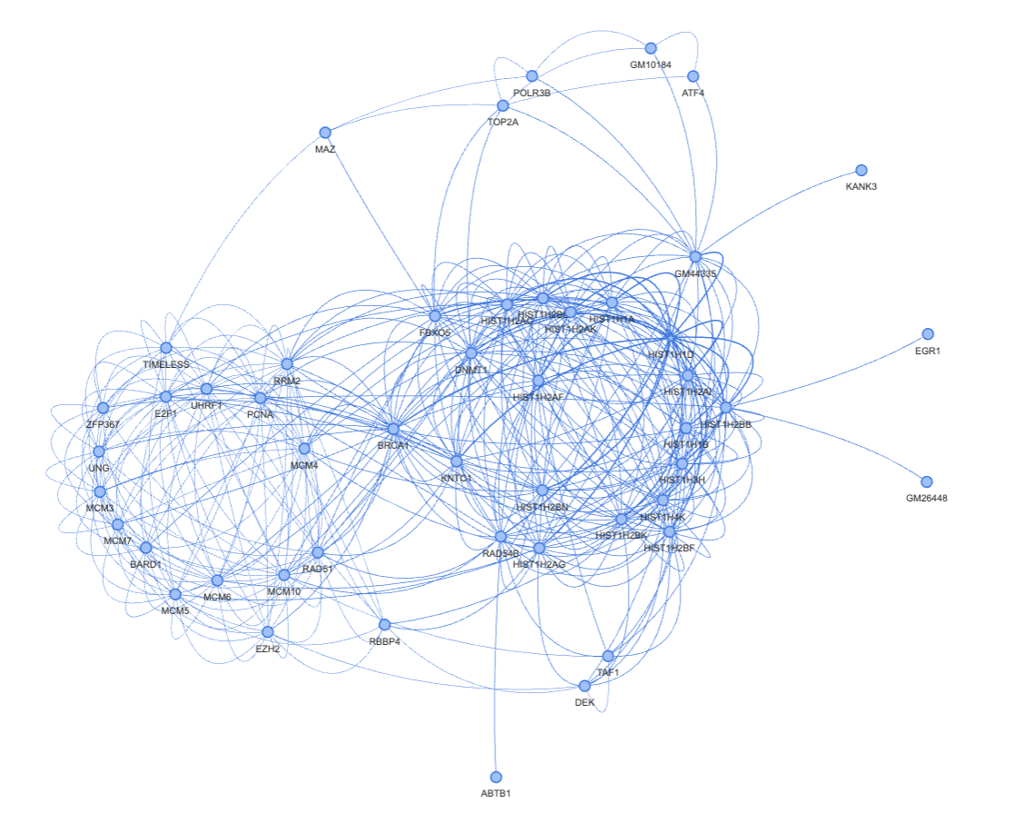
>>> g = grn.visualize_local_neighborhood(['HIST1H1D', 'MCM3'], k=40)
>>> g.show('view.html')

(Optional) Step 3. Node clustering

Here we have a fairly obvious bipartisan graph. It also makes sense to use some clustering methods to automatically assign nodes into partitions. You can use any clustering methods that you like (and works). Here is an example of using node2vec for this task.

>>> import networkx as nx
>>> from sklearn.cluster import KMeans
>>> from node2vec import Node2Vec
>>> 
>>> adj_table = grn.extract_local_neighborhood('HIST1H1D', 40)
>>> nxg = nx.from_pandas_edgelist(adj_table)
>>> 
>>> node2vec = Node2Vec(nxg, dimensions=64, walk_length=30, num_walks=200, 
>>>                     workers=4, seed=123)
>>> model = node2vec.fit(window=10, min_count=1, batch_words=4)
>>> 
>>> node_embeddings = [model.wv.get_vector(str(node)) for node in nxg.nodes()]
>>> 
>>> kmeans = KMeans(n_clusters=4, random_state=0).fit(node_embeddings)
>>> node_labels = kmeans.labels_
>>> 
>>> print("Clusters:")
>>> for cluster_id in range(max(node_labels) + 1):
>>>     cluster_nodes = [g for g, c in zip(
>>>         nxg.nodes(), node_labels) if c == cluster_id]
>>>     print(f"Cluster {cluster_id}: {','.join(cluster_nodes)}")
Clusters:
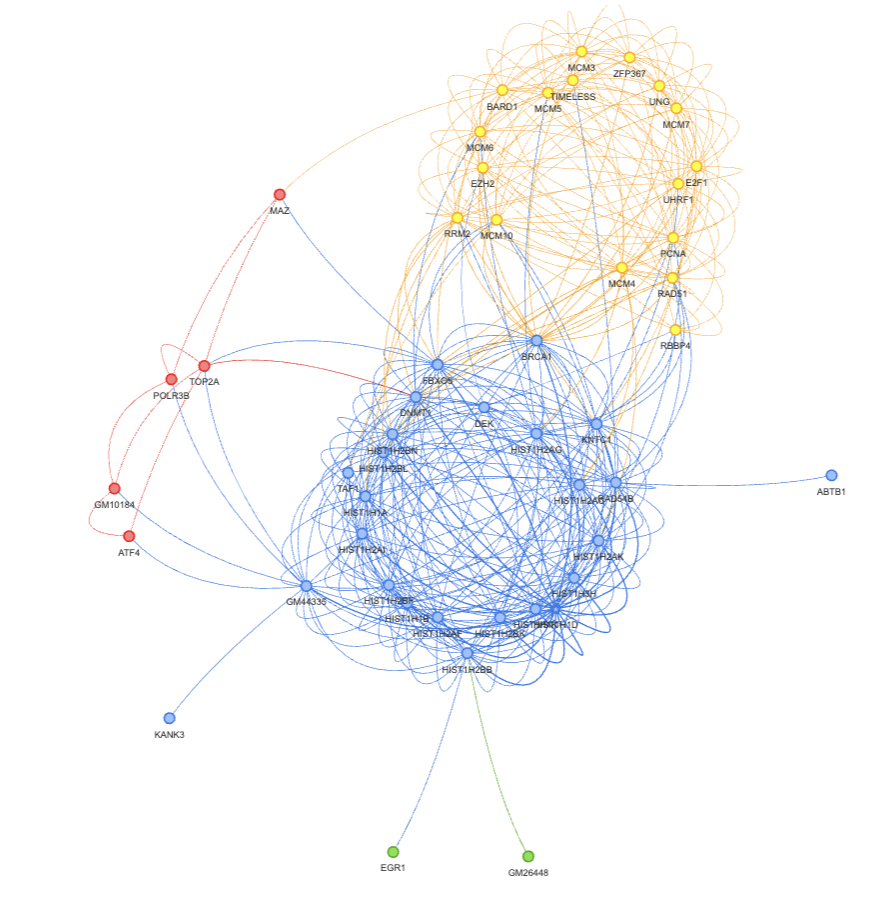
Cluster 0: HIST1H1D,HIST1H2BN,HIST1H2BK,HIST1H1B,HIST1H2BL,HIST1H2AK,HIST1H1A,HIST1H2AC,HIST1H2BF,HIST1H4K,HIST1H3H,HIST1H2AF,HIST1H2AI,HIST1H2AG,HIST1H2BB,DNMT1,BRCA1,KNTC1,RAD54B,GM44335,FBXO5,TAF1,ABTB1,DEK,KANK3
Cluster 1: MCM10,TIMELESS,RAD51,RBBP4,RRM2,MCM6,PCNA,E2F1,UHRF1,MCM4,MCM5,UNG,MCM7,MCM3,ZFP367,EZH2,BARD1
Cluster 2: TOP2A,MAZ,POLR3B,GM10184,ATF4
Cluster 3: GM26448,EGR1

You can also apply the clustering information to your visual.

>>> gene_group_dict = dict()
>>> gene_group_dict = {g:str(c) for g, c in zip(nxg.nodes(), node_labels)}
>>> g = grn.visualize_local_neighborhood(
>>>     'HIST1H1D', k=40, node_group_dict=gene_group_dict
>>>     )
>>> g.show('view.html')

Result Interpretation

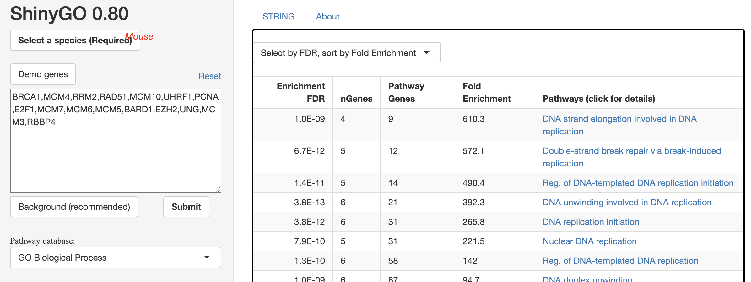
In the figure below, we clearly see two clusters. Most of the genes on the right side are obviously histone related since they all start with HIST. Genes on the left side are not that obvious. Therefore, we did a GO enrichment analysis on this gene set using shinyGo 0.80 and found that they are closely related to DNA replication and double strand break repair.

Recall that the mESC data comes from mouse embryonic stem cells, whose core functionality is replication. We believe this region of GRN represents the interaction between the core gene set of embryonic cells and histone related genes.

An interesting finding is that gene BRCA1 sits right in the middle of the core gene group and the histone group. It suggests that BRCA1 might play a role between histone and replication. In fact, we found a 2023 publication to support this hypothesis.