Fast SCENIC GRN Analysis with RegDiffusion#
Author: Nicky-Jin, edited by Hao
This tutorial demonstrates how to integrate GRN inference results from RegDiffusion into the SCENIC pipeline (Aibar 2017) for downstream gene regulatory network (GRN) analysis. In this workflow, RegDiffusion replaces GRNBoost2 (or GENIE3) by providing a much faster method to generate the adjacency matrix of the regulatory network. We then use PySCENIC’s pruning, cell scoring, and downstream visualization tools on the output of RegDiffusion.
Introduction#
SCENIC (Aibar 2017) is a widely used pipeline for inferring and analyzing GRNs in single-cell transcriptomics. Typically, its workflow consists of the following stages:
GRN inference: Done by GRNBoost2 or GENIE3.
Pruning: Refines co-expression modules using cisTarget to retain genes with TF-binding motifs.
Cell Scoring: Quantifies TF activity in individual cells via AUCell, a score measuring the activity of regulons.
Clustering and Visualization: The AUCell scores could be used as features to do dimension reduction and cell type identification.
One limitation with the default SCENIC pipeline is that the matrix calculation step with GRNBoost2 and GENIE3 is computationally intensive. Today, As the sizes of single-cell datasets continue to grow, running the SCENIC pipeline with default settings is becoming increasingly challenging. RegDiffusion offers a fast alternative with a deep-learning based denoising diffusion structural equation model (SEM). It can seamlessly replace the output from GRNBoost2/GENIE3 and reduce the computing time from hours to minutes or even seconds.
Prerequisites and Data Preparation#
pyscenic has some version conflicts with the latest packages and it may trigger some runtime error when performing specific tasks. We recommend setting up a separate conda environement to hold it. The following versions on the dependencies work well for us today (2025.3).
>>> conda create -y -n pyscenic-env python=3.10
>>> conda activate pyscenic-env
>>> pip install pyscenic==0.12.1 numpy==1.23.5 pandas==1.3.5 dask==2023.10.0 matplotlib decorator==4.3.0
>>> conda deactivate
You also need to install pyscenic to your working environment. We recommand the github version.
>>> pip install git+https://github.com/aertslab/pySCENIC
Data Sources#
Single-cell transcriptomic data#
For this tutorial, we use the mice lung dataset from GSE276682 (https://www.ncbi.nlm.nih.gov/geo/query/acc.cgi?acc=GSE276682) (Wu, 2025). This data includes a control group (n=3) and an intervention group (n=3). In the intervention group, mices were administered with intraperitoneal injection of 30mg/ml lipopolysaccharide (LPS) in saline to induce acute lung injury.
The raw FASTQ data was processed with cellranger to generate expression matrix. The count matrix was then processed following standard scanpy procedure and we focused on genes expressed in at least 5 cells. The input data has 55,129 cells and 3,701 genes.
Most of this tutorial is to illustrate the process. If you need access to the processed data, please download it from this link.
Auxiliary datasets for PySCENIC#
To run pySCENIC, you also need a set of auxiliary files. We recommend following the offical tutorial and download it from the official website. Basically, you would expect to download the following species-specific files.
The whole genome: https://resources.aertslab.org/cistarget/databases/
Motif to TF annotations database: https://resources.aertslab.org/cistarget/motif2tf/
For this tutorial, since we are working with mice, you will need to download the following files:
GRN Inference#
To get started, we first load the data and perfrom necessary data cleaning.
>>> import numpy as np
>>> import pandas as pd
>>> import scanpy as sc
>>> import regdiffusion as rd
>>> import loompy as lp
>>> from pyscenic.rss import regulon_specificity_scores
>>> from pyscenic.plotting import plot_rss
>>> import matplotlib.pyplot as plt
>>> import seaborn as sns
>>> sns.set_theme(style="white")
>>>
>>> # Change the path if needed
>>> wd = '../..'
>>> mice_data_path = f'{wd}/samples_cluster_ann.h5ad'
>>> cisdb_path = f'{wd}/mm10_10kbp_up_10kbp_down_full_tx_v10_clust.genes_vs_motifs.rankings.feather'
>>>
>>> # Load data. Data shape: 55,129 x 3701.
>>> adata = sc.read_h5ad(mice_data_path)
>>>
>>> # Filter the gene not present in the cisTargetDB. Data shape: 55,129 x 3,206
>>> cisdb = pd.read_feather(cisdb_path)
>>> adata = adata[:, adata.var_names.isin(cisdb.columns)]
>>> adata
View of AnnData object with n_obs × n_vars = 55129 × 3206
    obs: 'sample', 'cellname', 'celltype'
    var: 'mt', 'ribo', 'hb'
    uns: 'X_name'
    obsm: 'X_pca', 'X_pca_harmony', 'X_umap'
    varm: 'PCs'
    layers: 'counts'
    obsp: 'connectivities', 'distances'
The input of regdiffusion is log transformed raw counts data. The .X in the provided file has been normalized so we need to starts from the counts layer.
>>> # .X has been normalized so we need to get from the counts layer.
>>> # Counts is stored in a sparse matrix so we need to turn it to an array and
>>> # then perform log + 1 transformation.
>>> x = adata.layers["counts"].toarray()
>>> x = np.log(x+1.0)
Now run RegDiffusionTrainer. On NVIDIA A30 (24G), it took 19s. On A2000 (6G), it took 51s.
>>> rd_trainer = rd.RegDiffusionTrainer(x)
>>> rd_trainer.train()
Training loss: 0.221, Change on Adj: -0.000: 100%|██████████| 1000/1000 [00:19<00:00, 50.85it/s]
Extract edges from GRN#
The inferred GRN is represented by a weighted adjacency matrix and we would like to remove those weak edges. Here we recommend 2 strategies to do that. You can use either one of them or both depending on your need.
Focus on the top x% of edges based on the inferred weights. To do that you can use the
top_gene_percentileoption when you create an GRN object. Alternatively, after a GRN object is created, you can use theremove_weak_edgesand remove edges based on a manually specified threshold.For each gene, focus on the top-k regulator/targets. This is in fact the default way of getting edges in GENIE3. In
regdiffusion, once you have your GRN object, you can specifykin theextract_edgelistmethod of a GRN object (By default, k=20. If you want to extract all edges, you can set k=-1).
>>> # Now we focus on edges with weight > 50 percentile.
>>> grn = rd_trainer.get_grn(adata.var_names, top_gene_percentile=50)
>>>
>>> # Here for each gene, we are going to extract all edges
>>> edgelist = grn.extract_edgelist(k=-1, workers=4)
>>> edgelist.columns = ['TF', 'target', 'importance']
>>> edgelist.to_csv(f'{wd}/grn_naive.tsv', sep='\t', index=False)
>>>
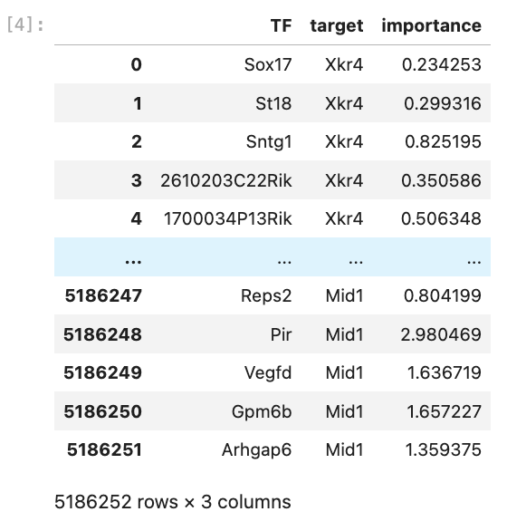
>>> # check edgelist.
>>> edgelist
You also need to save the expression matrix for pyscenic in the next step.
>>> lp.create(
>>>     filename=f'{wd}/exp_mtx.loom',
>>>     layers={"": x.transpose()},
>>>     row_attrs={"Gene": list(adata.var_names)},
>>>     col_attrs={"CellID": list(adata.obs_names)}
>>> )
Prunning and AUCell Calculation in PySCENIC#
In this step, we are going to call pyscenic from command line to prune the edges and generate the AUCell Scores for each individual cell. The whole process may take 5-20 minutes.
>>> ## inputs
>>> grn_fp=f'{wd}/grn_naive.tsv'
>>> exp_mtx_fp=f'{wd}/exp_mtx.loom'
>>>
>>> ## outputs
>>> ctx_output=f'{wd}/ctx_output.tsv'
>>> aucell_output=f'{wd}/aucell.loom'
>>>
>>> ## reference
>>> f_motif_path=f'{wd}/motifs-v10nr_clust-nr.mgi-m0.001-o0.0.tbl'
>>> f_db_500bp=f'{wd}/mm10_500bp_up_100bp_down_full_tx_v10_clust.genes_vs_motifs.rankings.feather'
>>> f_db_10kb=f'{wd}/mm10_10kbp_up_10kbp_down_full_tx_v10_clust.genes_vs_motifs.rankings.feather'
>>>
>>> ## Prunning. You may need to adjust the number of workers.
>>> !conda run -n pyscenic-env pyscenic ctx \
>>>     {grn_fp} \
>>>     {f_db_500bp} {f_db_10kb} \
>>>     --annotations_fname {f_motif_path} \
>>>     --expression_mtx_fname {exp_mtx_fp} \
>>>     --output {ctx_output} \
>>>     --num_workers 64
>>> ## AUCell Calculation
>>> !conda run -n pyscenic-env pyscenic aucell {exp_mtx_fp} \
>>>     {ctx_output} \
>>>     --output {aucell_output} \
>>>     --num_workers 64
2025-03-26 11:43:14,528 - pyscenic.cli.pyscenic - INFO - Creating modules.
2025-03-26 11:43:16,110 - pyscenic.cli.pyscenic - INFO - Loading expression matrix.
2025-03-26 11:43:18,362 - pyscenic.utils - INFO - Calculating Pearson correlations.
...
2025-03-26 11:47:11,450 - pyscenic.prune - INFO - Worker mm10_500bp_up_100bp_down_full_tx_v10_clust.genes_vs_motifs.rankings(4): Done.
2025-03-26 11:47:11,450 - pyscenic.prune - INFO - Worker mm10_500bp_up_100bp_down_full_tx_v10_clust.genes_vs_motifs.rankings(4): Done.
2025-03-26 11:47:11,521 - pyscenic.cli.pyscenic - INFO - Writing results to file.

Create regulons from a dataframe of enriched features.
Additional columns saved: []
2025-03-26 11:47:20,539 - pyscenic.cli.pyscenic - INFO - Loading expression matrix.
2025-03-26 11:47:22,420 - pyscenic.cli.pyscenic - INFO - Loading gene signatures.
2025-03-26 11:47:22,722 - pyscenic.cli.pyscenic - INFO - Calculating cellular enrichment.
2025-03-26 11:47:34,316 - pyscenic.cli.pyscenic - INFO - Writing results to file.
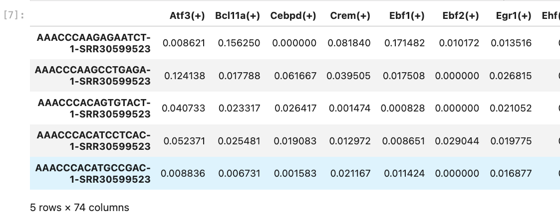
Once it’s finished, you can check the calculated AUCell values for each cell.
>>> lf = lp.connect(aucell_output, mode="r+", validate=False)
>>> auc_mtx = pd.DataFrame(lf.ca.RegulonsAUC, index=lf.ca.CellID)
>>> lf.close()
>>> auc_mtx.head()
Dimension reduction and cell type identification.#
Following the AUCell calcuation, UMAP can be used to perform additional dimensionality reduction for cell type identification.
>>> adata.obsm['X_aucell'] = auc_mtx.values
>>> sc.pp.neighbors(adata, n_neighbors=15, metric="correlation", use_rep="X_aucell")
>>> sc.tl.umap(adata)
>>> adata.obsm["X_aucell_umap"] = adata.obsm["X_umap"].copy()
>>>
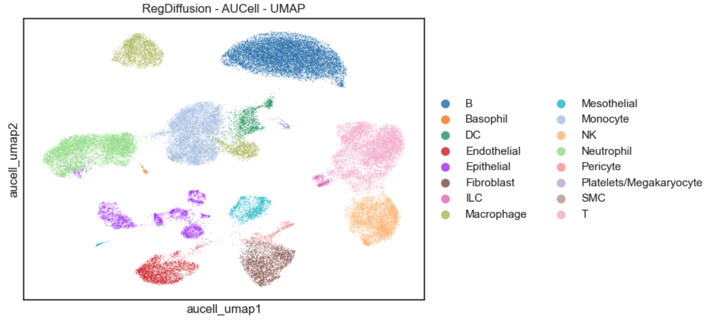
>>> sc.pl.scatter( adata, basis='aucell_umap',
>>> color=['celltype'],
>>> title=['RegDiffusion - AUCell - UMAP'],
>>> alpha=0.8
>>> )
We can compare the results with standard PCA-based UMAPs.
>>> sc.pp.neighbors(adata, n_neighbors=15, n_pcs=50, use_rep="X_pca")
>>> sc.tl.umap(adata)
>>> adata.obsm["X_pca_umap"] = adata.obsm["X_umap"].copy()
>>>
>>> # Remove batch effect with Harmony
>>> #!pip install harmonypy
>>> #sc.external.pp.harmony_integrate(adata, key = "sample")
>>> sc.pp.neighbors(adata, n_neighbors=15, n_pcs=50, use_rep="X_pca_harmony")
>>> sc.tl.umap(adata)
>>> adata.obsm["X_harmony_pca_umap"] = adata.obsm["X_umap"].copy()
>>>
>>> fig, axs = plt.subplots(1, 3, figsize=(18, 5))
>>>
>>> sc.pl.scatter(
>>>     adata, basis='pca_umap',
>>>     color='celltype',
>>>     title='PCA - UMAP',
>>>     alpha=0.8, ax=axs[0], show=False
>>> )
>>>
>>> sc.pl.scatter(
>>>     adata, basis='harmony_pca_umap',
>>>     color='celltype',
>>>     title='Harmony - PCA - UMAP',
>>>     alpha=0.8, ax=axs[0], show=False
>>> )
>>>
>>> sc.pl.scatter(
>>>     adata, basis='aucell_umap',
>>>     color='celltype',
>>>     title='RegDiffusion - AUCell - UMAP',
>>>     alpha=0.8, ax=axs[0], show=False
>>> )
>>>
>>> axs[0].get_legend().remove()
>>> axs[1].get_legend().remove()
>>>
>>> plt.tight_layout()
>>> plt.show()
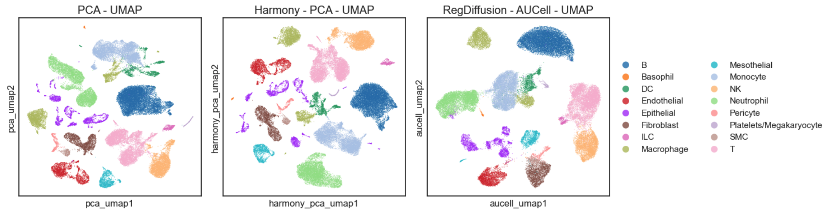
The RegDiffusion-AUCell-based UMAP plot provides a high degree of clarity, allowing the major cell types to be easily distinguished. Compared with standard PCA-based UMAPs, whether or not batch effects are corrected with harmonypy, the AUCell plot produces fewer, more distinctly separated clusters. This clear separation remains interpretable even in the absence of cell labels, which suggests its capacity for identifying novel cell subtypes.
>>> label_dict = {
>>>     "SRR30599518": "CTL-1",
>>>     "SRR30599519": "CTL-2",
>>>     "SRR30599520": "CTL-3",
>>>     "SRR30599521": "LPS-1",
>>>     "SRR30599522": "LPS-2",
>>>     "SRR30599523": "LPS-3"
>>> }
>>> adata.obs['label'] = [label_dict[x] for x in adata.obs['sample']]
>>> fig, axs = plt.subplots(1, 3, figsize=(13, 4))
>>>
>>> sc.pl.scatter( adata, basis='pca_umap',
>>>     color=['label'],
>>>     title=['PCA - UMAP'],
>>>     alpha=0.9, ax=axs[0], show=False, palette='RdYlBu'
>>>     )
>>>
>>> sc.pl.scatter( adata, basis='harmony_pca_umap',
>>>     color=['label'],
>>>     title=['Harmony - PCA - UMAP'],
>>>     alpha=0.9, ax=axs[1], show=False, palette='RdYlBu'
>>>     )
>>>
>>> sc.pl.scatter( adata, basis='aucell_umap',
>>>     color=['label'],
>>>     title=['RegDiffusion - AUCell - UMAP'],
>>>     alpha=0.9, ax=axs[2], show=False, palette='RdYlBu'
>>>     )
>>>
>>> axs[0].get_legend().remove()
>>> axs[1].get_legend().remove()
>>>
>>> plt.tight_layout()
>>> plt.show()
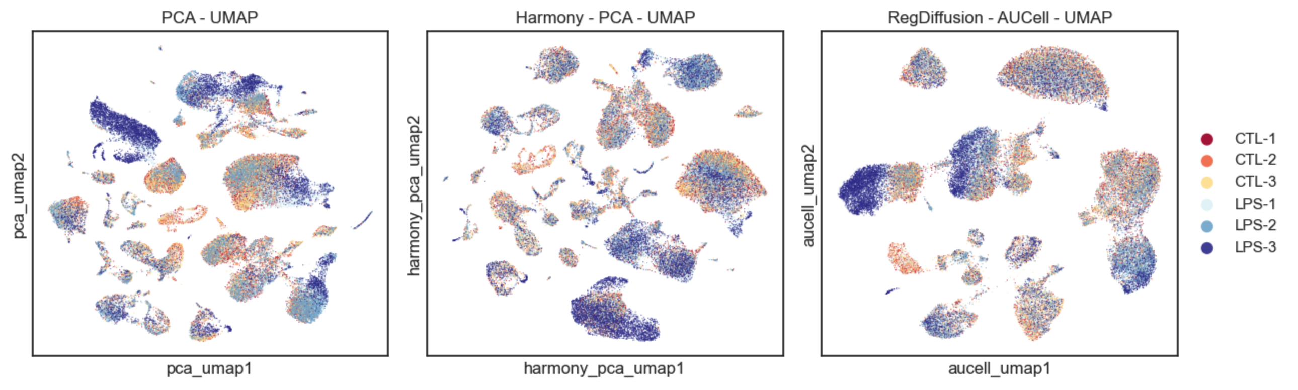
To assess the impact of batch effects, we colored the UMAP plots using sample labels. As shown in the figure above, Harmony effectively reduced sample differences across many cell types. Similarly, in the RegDiffusion-AUCell UMAP, batch effects were also minimized, resulting in a near-uniform distribution of data points. This consists with previous literature (Aibar, 2017; Malagola, 2024) and shows that AUCell scores effectively capture high-level interaction features. Interestingly, as the batch effect was diminished, the biological effects were revealed more intuitively. For example, we can see clear separations in Neutrophils from samples in the LPS group and in the control group, which is consistent with previous studies demonstrating that emergency granulopoiesis leads to different clusters of neutrophils during sepsis. In contrast, these patterns appear to be lost when the data is processed with Harmony.
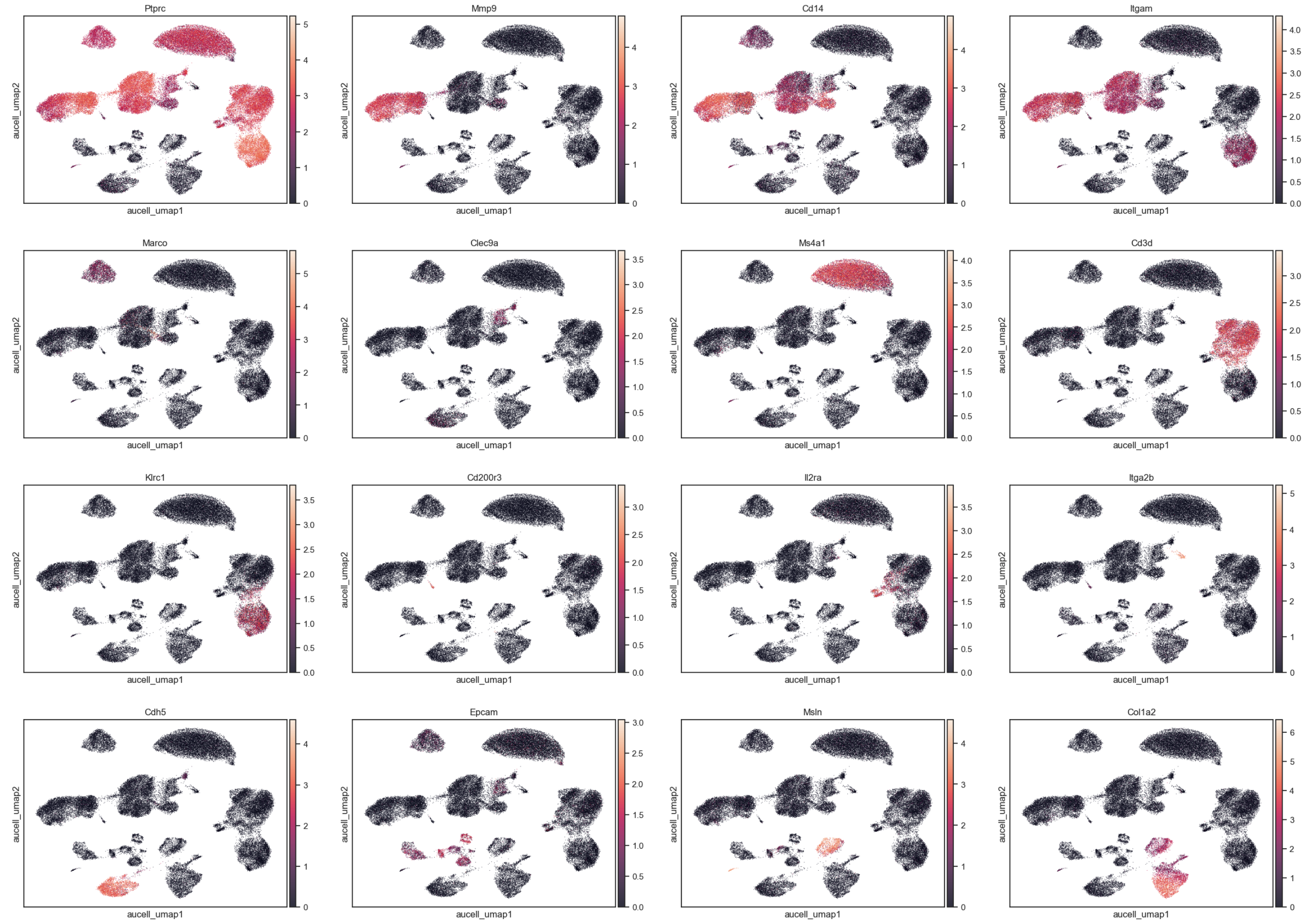
Expression levels of Bio-markers#
markers= ['Ptprc',
          'Mmp9', # Neutrophil
          'Cd14', 'Itgam',  # Monocyte
          'Marco',  # Macrophage
          'Clec9a',  # DC
          'Ms4a1', # B
          'Cd3d', # T
          'Klrc1',  # NK
          'Cd200r3',  # Basophil
          'Il2ra', # ILC
          'Itga2b', # Platelets
          'Cdh5', # Endothelial
          'Epcam', # Epithelial
          'Msln', # Mesothelial
          'Col1a2' # Mesenchymal cells
]

sc.pl.embedding(
    adata, basis='aucell_umap',
    color=markers,
    ncols=4, alpha=0.8
)
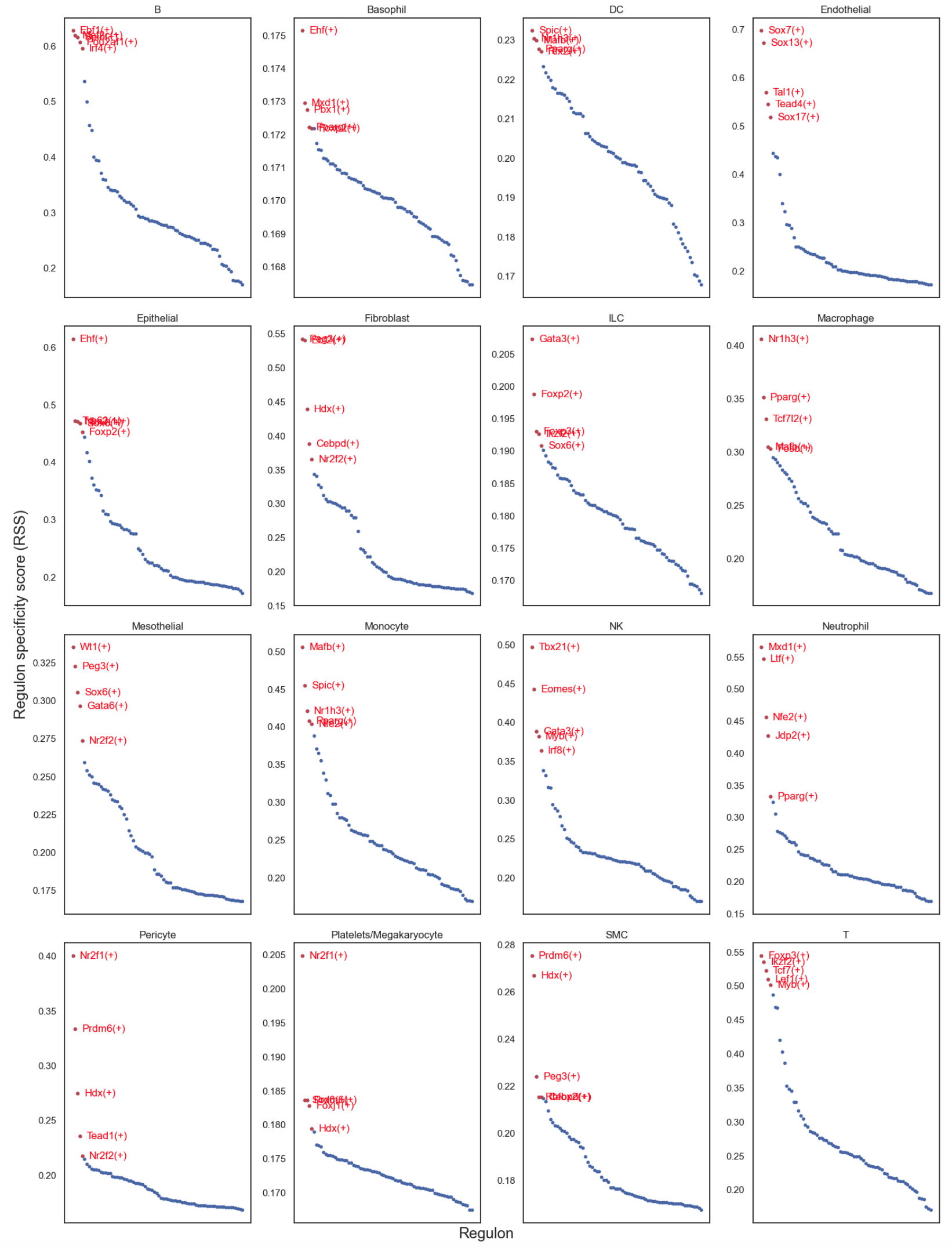
Regulon specificity scores by cell types#
>>> rss = regulon_specificity_scores(auc_mtx, adata.obs.celltype)
>>> cats = sorted(list(set(adata.obs['celltype'])))
>>>
>>> fig = plt.figure(figsize=(15, 20))
>>> for c,num in zip(cats, range(1,len(cats)+1)):
>>>     x=rss.T[c]
>>>     ax = fig.add_subplot(4,4,num)
>>>     plot_rss(rss, c, top_n=5, max_n=None, ax=ax)
>>>     ax.set_ylim( x.min()-(x.max()-x.min())*0.05 , x.max()+(x.max()-x.min())*0.05 )
>>>     for t in ax.texts:
>>>         t.set_fontsize(12)
>>>     ax.set_ylabel('')
>>>     ax.set_xlabel('')
>>>
>>> fig.text(0.5, 0.0, 'Regulon', ha='center', va='center', size='x-large')
>>> fig.text(0.00, 0.5, 'Regulon specificity score (RSS)', ha='center', va='center', rotation='vertical', size='x-large')
>>> plt.tight_layout()
>>> plt.rcParams.update({
>>>     'figure.autolayout': True,
>>>         'figure.titlesize': 'large' ,
>>>         'axes.labelsize': 'medium',
>>>         'axes.titlesize':'large',
>>>         'xtick.labelsize':'medium',
>>>         'ytick.labelsize':'medium'
>>>         })
>>> plt.show()
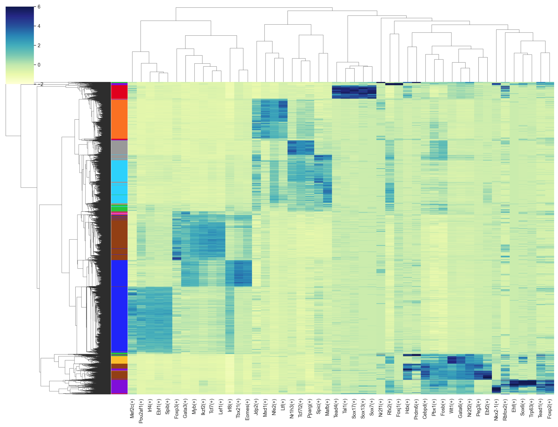
Heatmap#
>>> # Top 5 regulons for each cell type
>>> topreg = []
>>> for i,c in enumerate(cats):
>>>     topreg.extend(
>>>         list(rss.T[c].sort_values(ascending=False)[:5].index)
>>>     )
>>> topreg = list(set(topreg))
>>>
>>> # Normalized z scores
>>> auc_mtx_Z = pd.DataFrame( index=auc_mtx.index )
>>> for col in list(auc_mtx.columns):
>>>     auc_mtx_Z[ col ] = ( auc_mtx[col] - auc_mtx[col].mean()) / auc_mtx[col].std(ddof=0)
>>>
>>> # Heatmap
>>> def palplot(pal, names, colors=None, size=1):
>>>     n = len(pal)
>>>     f, ax = plt.subplots(1, 1, figsize=(n * size, size))
>>>     ax.imshow(np.arange(n).reshape(1, n),
>>>               cmap=matplotlib.colors.ListedColormap(list(pal)),
>>>               interpolation="nearest", aspect="auto")
>>>     ax.set_xticks(np.arange(n) - .5)
>>>     ax.set_yticks([-.5, .5])
>>>     ax.set_xticklabels([])
>>>     ax.set_yticklabels([])
>>>     colors = n * ['k'] if colors is None else colors
>>>     for idx, (name, color) in enumerate(zip(names, colors)):
>>>         ax.text(0.0+idx, 0.0, name, color=color, horizontalalignment='center', verticalalignment='center')
>>>     return f
>>>
>>> colors = sns.color_palette('bright',n_colors=len(cats) )
>>> colorsd = dict(zip( cats, colors ))
>>> colormap = [colorsd[x] for x in adata.obs['celltype']]
>>>
>>> sns.set(font_scale=1.2)
>>> g = sns.clustermap(auc_mtx_Z[topreg], annot=False,  square=False,  linecolor='gray',
>>>     yticklabels=False, xticklabels=True, vmin=-2, vmax=6, row_colors=colormap,
>>>     cmap="YlGnBu", figsize=(21,16) )
>>> g.cax.set_visible(True)
>>> g.ax_heatmap.set_ylabel('')
>>> g.ax_heatmap.set_xlabel('')
References#
Aibar, S., et al. 2017. SCENIC: single-cell regulatory network inference and clustering. Nat Methods 14, 1083–1086. https://doi.org/10.1038/nmeth.4463
Malagola, E., et al. 2024. Isthmus progenitor cells contribute to homeostatic cellular turnover and support regeneration following intestinal injury. Cell 187, 3056-3071.e17. https://doi.org/10.1016/j.cell.2024.05.004
Wu, M., Wang, S., Chen, X., Shen, L., Ding, J., Jiang, H., 2025. Single-cell transcriptome analysis reveals cellular reprogramming and changes of immune cell subsets following tetramethylpyrazine treatment in LPS-induced acute lung injury. PeerJ 13, e18772. https://doi.org/10.7717/peerj.18772